Recent advances in Bayesian inference of isolation-with-migration models
Article information

Abstract
Isolation-with-migration (IM) models have become popular for explaining population divergence in the presence of migrations. Bayesian methods are commonly used to estimate IM models, but they are limited to small data analysis or simple model inference. Recently three methods, IMa3, MIST, and AIM, resolved these limitations. Here, we describe the major problems addressed by these three software and compare differences among their inference methods, despite their use of the same standard likelihood function.
Introduction
Divergence between populations and species has been a major interest in population genetics and evolution. Estimating divergence from genetic data is difficult because of conflicting evolutionary processes. Genetic drift elevates divergence between populations or between species, while gene flow can remove signals of divergence [1]. An isolation-with-migration (IM) model is a widely used demographic model describing the two conflicting signals. A typical 2-population IM model with six parameters (Fig. 1) depicts two populations (sizes θ1 and θ2, respectively) that arise from a single ancestral population (size θa) at time TS in the past, while the two populations may exchange migrants at rates m1 and m2 ([1-3] for notations). Both population sizes and migration rates are assumed to be constant over time [4].

Isolation-with-migration model with six demographic parameters.
The challenges of inferring isolation models (with no migrations) and even phylogeny have been addressed by using a multispecies coalescent framework [5-11]. However, ignoring migrations can result in a biased estimation of splitting times of populations/species and may lead to a wrong phylogenetic tree estimation [12-16]. Efforts to distinguish between isolation and migration began about 20 years ago, and many methods have employed a Markov chain Monte Carlo (MCMC) simulation to infer an IM model [2-4,17-21]. However, most methods have a major roadblock of a long computational time of an MCMC simulation, which typically limits the amount of data that can be analyzed [1]. In addition, the joint estimation of both phylogeny and an IM model is known to be tremendously difficult [16].
Recently, three methods have been developed to address the scalability of the data and/or to jointly infer phylogeny in the presence of gene flow. IMa3 [16] is the most recent version of IM/IMa series software and infers the phylogeny and IM models. MIST [1] needs a known (or assumed) phylogeny but is able to analyze thousands of loci. AIM [14,22] is a package in the popular BEAST platform and also infers phylogeny in the presence of gene flow. Similar to other methods, these three methods implement the standard probabilistic framework and employ an MCMC simulation for inference.
The advent of many inference methods is not commensurate to our skills of analysis using those programs. In order to ensure the use of appropriate programs and to correctly interpret results, it is essential to understand the inference methods used and the results that the programs provide. IMa3, MIST, and AIM all use similar standard probabilistic models and apply Bayesian inference, but their inference strategies and the types of results may be different. Therefore, users must first understand the differences in their inference methods.
To elucidate the current state of the art in the analysis of IM models, in this review article, we compare the three methods and accompanying software, IMa3, MIST, and AIM (BEAST platform). In particular, the data type and the underlying model structures will be discussed, followed by a brief summary of an MCMC algorithm and mixing issue. Then, this review article will focus on comparison of the advanced methods: IMa3, MIST, and AIM. We do not intend to explain the basic concepts of standard probabilistic models and MCMC algorithms, but extensive reviews of them are available elsewhere [9,23-25].
DNA Alignments
One of the most common types of data used in the analysis of IM models and phylogeny is DNA sequence alignments. Most methods, including IMa3, MIST, and AIM, assume the alignments are correct, although they are estimated from models of insertions and deletions [26]. The relatedness of homologous DNA sequences is considered to the result from past branching processes, so the DNA sequence alignments must be orthologs [22]. Moreover, no selection but a neutral evolution is assumed to act on alignments. Since most methods typically assume that there is no recombination within a locus and free recombination between loci, alignments should not overlap or be closely located. Moreover, filtering using a four-gamete test [27] is essential to minimize potential recombination within a locus.
Standard Model Structure
When inferring an IM model from genetic data, the parameters of interest are demographic parameters of the IM model, denoted as a vector ψ=(θ1, θ2, θa, m1, m2, TS). The ith locus Di out of L loci are the observations, and the genealogy Gi of Di is a latent variable that we cannot observe typically (Fig. 2). Fig. 2 depicts the structure of the standard models. The standard models address two levels of uncertainty: the distribution of DNA sequences given genealogy and that of genealogy given an IM model [11,12,25]. We typically assume that there is no recombination within a locus and free recombination between loci. In other words, the ith locus Di out of L loci has as its own genealogy Gi and loci are independent. Given genealogy, the genetic data and demography ψ=(θ1, θ2, θa, m1, m2, TS) are assumed to be conditionally independent. As the distribution of DNA sequences
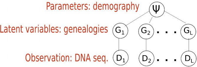
Standard model structure. Each locus has its own genealogy. Given genealogy, the genetic data and demography are assumed to be independent.
The likelihood function, so-called Felsenstein’s equation [35], does not have a general closed-form and is difficult to numerically evaluate [3].
MCMC Simulation and the Mixing Problem
A feasible way to numerically evaluate the likelihood function (Eq. 1) is an MCMC simulation. Extensive reviews of fundamental concepts, diverse algorithms, and MCMC diagnosis are available elsewhere [23,25,36,37]. With a prior distribution on ψ, the posterior density of ψ given data is
The target density of an MCMC simulation is
One of the benefits of such a simulation is an easy approximation of the marginal posterior density (Eq. 2) by making use of simulated values for the parameter of interest. For example,
A popular MCMC algorithm is a Metropolis-Hastings within Gibbs sampling algorithm (Fig. 3). Within each iteration, all demographic parameters and genealogies are sequentially simulated. For example, Fig. 4A shows the state of the (t-1)th iteration for the genealogy of one locus and all demographic parameters ψ including splitting time

A typical Metropolis-Hastings within Gibbs sampling algorithm.

An example of an Markov chain Monte Carlo step to update the splitting time TS. (A) The current state of genealogy and all demographic parameters, including TS. (B) A newly proposed splitting new TS, which is not compatible with the state of genealogy.
While samples via a traditional Monte Carlo method are independent, MCMC samplers generate autocorrelated draws because the current value is either a different value or the same as the previous. Strong autocorrelations slow down traversing the posterior space and take longer to produce independent-like samples ψt, … ψn ~
Inference Methods
IMa3
The software series of IM/IMa were developed to infer IM models (Table 1) [39,40]. The first software, called IM, analyzes either a single locus [4] or multiple loci [2], and implements MCMC approaches to infer six demographic parameters

Comparison of Bayesian software MIST, AIM, and IMa3 (IM/IMa series)
This yields a better mixing than software IM by reducing the number of parameters to sample, but it does not resolve the fundamental barrier of the relation between genealogies and splitting time. As a result of an MCMC simulation, the sampled values approximate the marginal posterior of the splitting time:
The most recent version called IMa3 modified the MCMC procedure of IMa2 to infer an IM model parameters as well as phylogeny [16], while IMa2 requires the phylogeny of multiple populations to be known. It is very difficult to co-estimate the phylogeny and IM model parameters, because sampling phylogeny together with IM parameters and genealogies also yields poor mixing. For example, a newly proposed phylogeny may not be compatible with the current state of migrations and is therefore rejected. IMa3 introduces pseudo-migrations, called “hidden migrations,” that occurred earlier than the splitting time so that a newly proposed splitting time or phylogeny is not instantly rejected but evaluated with non-zero acceptance probability. For example, if a newly proposed splitting time is younger than existing migrations (Fig. 4B), the migration paths older than splitting time are considered hidden migration paths (MH) and the genealogy is the one without hidden migrations and compatible with the new splitting time. In other words, the current genealogy, given the new splitting time, is a so-called “hidden genealogy” GH=(G, MH). Given phylogeny τ and demographic parameters ψ, the distribution of the hidden genealogy is partitioned into those of hidden migrations and the genealogy without hidden migrations:
Then τ1, ... , τn from the MCMC samples approximately follow the marginal posterior
MIST
Software MIST [1] implements a 2-step analysis. First, it simulates genealogies without migrations (so-called coalescent trees λ_) via an MCMC simulation. Note that no information about a demographic model is necessary in the first step, which alleviates the mixing problem. Second, the joint posterior density
Although MIST does not sample migrations and the underlying demographic model in step 1, the same posterior density
where the ith genealogy Gi=(λi, Mi)and Mi is the set of all migration information. This rewrites Eq. (2) as follows:
The exact computation of
As a result, MIST provides the MAP of all demographic parameters that maximize the joint posterior Eq. (6).
MIST has several strengths statistically and computationally. First, the computational complexity linearly increases with the number of loci. Analyses of thousands of loci do not give rise to mixing problems. Second, similar to IMa series, the approximate p(ψ│D) in Eq. (6) can be used for LRTs for migration rates. While the IM/IMa series uses the marginal
densities, MIST provides the joint distribution of all demographic parameters (Table 2). Since the estimations of demographic parameters are correlated, LRTs based on joint distributions have false-positive rates close to the expected value (e.g., 5%), even when very high false-positive rate occurred by LRTs based on marginal distributions [1,41,42]. Third, the importance sampling method enhances the computational efficiency for model comparisons. When different demographic models are compared, the simulated values from an MCMC simulation in step 1 can be repeatedly employed to infer different demographic models in step 2.

Prior assumptions, migration rate tests and scalability of Bayesian software MIST, IMa3, and AIM
AIM
AIM [14] implements a Bayesian inference of phylogeny and IM models in using the BEAST platform [15,43]. BEAST is a software platform for phylogenetic analyses, phylodynamics, and population genetics. starBEAST2 [44], an extended BEAST package, was added to estimate species trees in the absence of gene flow. AIM was recently added to estimate the posterior density
where L1 and L2 are lineages of λ at time t. AIM implements this independence approximation rather than the exact density
AIM reparamerized migration rates as follows: migration rate between populations A and B,
AIM performs tests for migration rates based on Bayes factors (BFs) [14], while IMa3 and MIST use LRTs (Table 2). A BF as the ratio of marginal likelihoods [37] is wildely used for model selection. Since AIM is a package in the BEAST platform, users can take advantage of other existing packages and MCMC diagnostic tools. However, most packages in BEAST were developed independently [15,45]. Therefore, the results provided by different packages are not connected, and users need to be aware of the different terminologies by each package [15].
Discussion
IMa3, MIST, and AIM are advanced software that estimate demographic parameters of IM models. IMa3 and AIM sample population tree topologies and all or partial demographic parameters through an MCMC simulation. Therefore, their estimations are based on the marginal posterior distribution of parameters. MIST can estimate the joint posterior distribution of all parameters, thereby providing a joint estimation. IMa3 and AIM estimate population tree topology and migration rates, but their scalability to genomic data is limited or has not been yet examined. MIST scales well with genomic data and can be extended to infer population tree topologies. However, the software currently supports a joint estimation of demographic parameters of 2-population IM models.
While AIM uses BFs for migration rate test, IMa3 and MIST suggest LRTs. While IMa3 compares marginal posterior distributions, MIST provides joint posterior distributions for LRTs. When splitting times are recent, it is important to consider using joint distributions for LRTs in order to avoid a high false-positive [1,41,42].
Long-standing barriers to inferring IM models have been resolved by IMa3, MIST, and AIM. MIST can analyze genome-scale data without sever mixing problems in an MCMC simulation. IMa3 and AIM are able to estimate IM models and phylogeny in the presence of migrations. Nonetheless, there are still unresolved questions and no software implementing sophisticated models to answer the questions. One of the major interests for the future is to relax the strong assumption of constant migration rates and population sizes over time. Current methods that attempt to solve this problem are limited to small data or not capable of inferring IM models from real genetic data analysis [46,47].
Notes
Conflicts of Interest
No potential conflict of interest relevant to this article was reported.
Acknowledgements
This work was supported by the National Research Foundation of Korea (NRF) grant funded by the Korea government (MSIT) (No. NRF-2018R1C1B5044541).