

Introduction
Various proteins interact with DNA in the nucleus. These interactions include many essential cellular processes, such as DNA replication, recombination, repair, transcription, and histone modifications [1]. Recent works have established that the eukaryotic chromatin is a dynamic and complex assembly of DNA, RNA, and proteins and is regulated by various post-translational modifications, including histone modifications, DNA methylation, long-range interactions, and non-coding RNAs [2]. The development of chromatin immunoprecipitation combined with chip or sequencing (ChIP-chip and later ChIP-Seq) has provided powerful methods to elucidate the complex interaction between DNA and proteins in the nucleus and has produced interesting data on complex DNA-protein interactions in the cell. By allowing genomewide analysis of DNA-protein interactions and histone modifications, ChIP-Seq has become one of the essential methods for genomic and epigenomic research.
Along with the development of ChIP-Seq data generation methods, various algorithms, methods, and tools have been developed for various steps during ChIP-Seq data analysis. Now, the standard ChIP-Seq data analysis process consists of a quality check (QC), mapping, peak calling, statistical analysis, annotation, and visualization. There are several well-known tools for these steps: ‘Trim Galore’ is one of the best programs to trim fastq reads, and ‘FastQC’ is also one of the major tools for quality control and pre-processing of fastq files. These tools are found at http://www.bioinformatics.babraham.ac.uk/projects/. Bowtie and bwa are two representative tools for read mapping [3,4]. For peak calling, MACS2 is one of the most widely used tools in ChIP-Seq data analysis [5]. ‘MAnorm’ can be conveniently used for statistical analysis of ChIP-Seq data [6], and ‘PAVIS’ is available for biological interpretation of ChIP-Seq peaks in a user-friendly web interface [7]. While many tools have been developed for ChIP-Seq data analysis, no tool can provide all the necessary steps of ChIP-Seq data analysis in one environment. Also, many of the ChIP-Seq analysis tools need Unix-like environments (e.g., UNIX/LINUX or Mac OS X); so, most users of the Windows operating system have difficulty in using them.
The Bioconductor project, which was launched in 2001, now contains more than 2,000 packages that facilitate the analysis and interpretation of high-throughput genomic data. As the Bioconductor project is based on the R statistical language, which is available for all of the major operating systems, most packages in Bioconductor can be run across different operating systems. In this regard, packages in the Bioconductor project provide an excellent platform for developing a streamlined analysis pipeline that can be run independently of platform. In this work, we selected four packages (dada2 [8], QuasR [9], mosaics [10], and ChIPseeker [11]) from the Bioconductor project, and made a ChIP-Seq data analysis pipeline that performs all the essential steps in one script. We hope that this example will help biologists with few bioinformatics skills in their analysis of ChIP-Seq data.
Methods
Public data download
While most researchers are likely to analyze their own data, some users may download public ChIP-Seq data from repositories, such as Short Read Archive (SRA) and the Encyclopedia of DNA Elements (ENCODE) project data portal. In this paper, we used a dataset from Gene Expression Omnibus (GSE29611; the data can be found at http://www.ebi.ac.uk/ena/data/view/SRP006944), one of the datasets from the ENCODE project [12], which aims to identify all functional elements in the human genome. Among the many samples in GSE29611, we used two samples from HeLa cells (Table 1).
Description of packages and testing environment
We used only four packages from beginning to end. The list of packages is shown in Table 2. The workflow in this paper was tested on a PC with an Intel i7 3.60 GHz processor and 16 GB memory using Microsoft R Open (version 3.3.0) in the Windows 8.1 pro K operating system.
Results
Setting the R environment and installing libraries to analyze (step 0 to step 1)
First, we provide a short R code to install the Bioconductor-based program. Next, it provides the ‘biocLite’ command to install the necessary package to analyze, the ‘setwd’ command to set up the working directory, and the ‘library’ command to load the package.
(Optional) Data download from public repository (step 2)
We downloaded two samples of the GSE29611 dataset from the European Bioinformatics Institute (EBI) database. We used EBI instead of SRA, as EBI provides both fastq and sra files, while SRA provides only sra files. By ftp protocol, it took about 45 min to download two fastq files from the EBI ftp site.
Trimming the sequencing file (step 3)
fastq file filtering is an important step when dealing with high-throughput sequencing data, because low-quality sequences can contain unexpected and misleading errors; especially, Illumina sequencing quality tends to drop off at the ends of reads, and the initial nucleotides can also be problematic due to calibration issues, such as trimming issues. The ‘dada2’ package can filter and trim a fastq file with the ‘fastqFilter’ function. ‘fastqFilter’ takes an input fastq file and filters it, based on several user-definable criteria, and outputs those reads that pass the filter and their associated qualities to a new fastq file. The main parameters of the ‘fastqfilter’ function are ‘fn’ and ‘fout,’ which indicate the path to the input fastq file and to the output file. Additionally, we adjusted the ‘compress’ option to ‘TRUE,’ because we use the compressed fastq file for analysis.
Sequence alignment (step 4)
The first step in ChIP-Seq data analysis is to align fastq files to a reference genome. The names of fastq files and the reference genome information (either a fasta file or BSgenome package) should be provided. As mapping is a time-consuming job, parallel processing using multiple cores is highly recommended. In R, parallel programming is supported by the 'BiocParallel' package, found at https://bioconductor.org/packages/release/bioc/html/BiocParallel.html. QuasR, the abbreviation for ‘Quantify and Annotate Short Reads,’ provides a framework for the quantification and analysis of short reads. ‘qAlign’ is the function that generates alignment files in BAM format for all input sequence files against the reference genome. The qAlign function is a wrapper for the bowtie [3] and SpliceMap [13] tools.
Quality check (step 5)
The next step after sequence alignment is the QC of the aligned reads. The QC is performed by the ‘qQCReport’ function of the qAlign package. It samples a random subset of sequences and alignments from each sample or an input file and generates a series of diagnostic plots for estimating data quality by various methods. The output consists of seven plots. The main plot is shown in Fig. 2, and the other six plots are shown in Supplementary Files (Fig. 2, Supplementary Figs. 1, 2, 3, 4, 5, 6).
Peak calling (step 6)
For ChIP-Seq peak calling, we chose the ‘mosaics’ package, which uses an adaptive and robust statistical approach; ‘mosaics’ is an acronym of “Model-Based One- and Two-sample Analysis and Inference for ChIP-Seq data.” It implements a flexible parametric mixture modeling approach for detecting peaks—e.g., enriched regions—in one-sample (ChIP sample) or two-sample (ChIP and matched control samples) ChIP-Seq data. It can account for mappability and GC content biases that arise in ChIP-Seq data [10]. Recently, ‘mosaics’ extended the framework with a hidden Markov Model (HMM) architecture, named mosaics-HMM [14], to identify broad peaks; so, mosaics is useful for the analysis of both sharp and broad peaks. As for broad peaks, mosaics has two methods: ‘mosaicsFitHMM’ and ‘mosaicsPeakHMM.’ For computational efficiency, ‘mosaicsFitHMM’ utilizes MOSAiCS model fit as estimates of emission distribution of the MOSAiCS-HMM model. In addition, it also considers MOSAiCS peak calling results at a specified false discovery rate (FDR) level as initial values by default. For more information, please peruse the vignette on 'mosaics' in Bioconductor. Here, we describe an example of a sharp peak calling process.
Calling of sharp peaks (steps 6-2 to 6-5)
For peak calling, mosaics first constructs bin-level files from aligned read files for modeling and visualization. The ‘infile’ argument indicates the name of the aligned files, and the ‘fileFormat’ argument indicates the data format of the ‘infile.’ Also, several arguments should be provided: ‘bychr,’ ‘PET,’ ‘fragLen,’ ‘binsize,’ and ‘capping.’ The meaning of each argument is given in ‘constructing separate bin-level file for each chromosome,’ ‘paired-end tag,’ ‘average fragment length,’ ‘size of bins,’ and ‘maximum number of reads allowed to start at each nucleotide position,’ respectively [10]. Then, binned data are read into the R environment. Here, for the ‘type’ argument, ‘input’ and ‘chip’ indicate either a control or ChIP-Seq data file, respectively. ‘readBins’ is a versatile function, which imports and preprocesses all or a subset of bin-level ChIP-Seq data, including ChIP data, matched control data, mappability score, GC content score, and sequence ambiguity score. The next step is to fit the MOSAiCS model. The ‘mosaicsFit’ function performs fitting of one-sample or two-sample MOSAiCS models with one signal component or two signal components. The ‘analysisType’ parameter uses ‘OS (one-sample analysis),’ ‘TS (two-sample analysis using mappability and GC content),’ or ‘IO (two-sample analysis without using mappability and GC content).’ The ‘bgEst’ parameter selects a background estimation approach from either ‘matchLow (estimation using bins with low tag counts)’ or ‘rMOM (estimation using robust method of moment).’ After model fitting, peaks are identified. The sharp peaks are identified by applying the two-signal component model at a given FDR. Here, the argument ‘signalModel=2S’ indicates the two-signal component model, while ‘signalModel=1S’ indicates the one-signal component model. The FDR can be controlled at the desired level by specifying the ‘FDR’ argument. Initial nearby peaks are merged if the distance (bp) between them is less than maxgap on the argument ‘maxgap.’ The ‘minsize’ argument sets a threshold to remove peaks whose width is narrower than the given value. ‘thres’ sets a threshold for ChIP tag counts for peaks. Called peaks can be exported in diverse file formats, including the TXT, BED, GFF, narrow-Peak, and BroadPeak file formats.
Calling of broad peaks (Supplementary Methods)
We provide another version of R code for calling broad peaks (Supplementary Methods, Supplementary Figs. 7, 8, 9, 10, 11).
Annotation and visualization (step 7)
The main input format for the ChIPSeeker package [13] is a bed file. ‘readPeakFile’ reads data from the input file and stores them in a data.frame or Granges object.
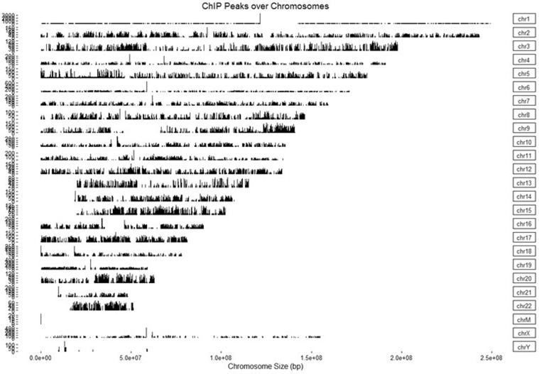
ChIP peaks coverage plot (Step 7-2)
The ‘Covplot’ function calculates the coverage of peak regions over chromosomes and generates a figure (Fig. 3). The ‘weightCol’ argument indicates the peak score, and ‘V5’ means the fifth column.
Heatmap and average profiling of chip peaks binding to transcription start site regions (Fig. 4A and 4B) (step 7-3)
First, transcription start site (TSS) regions are prepared by invoking the ‘getPromoter’ function. Then, peaks are mapped to the TSS regions, generating tagMatrix. The ‘tagHeatmap’ function plots the heatmap based on the tagMatrix data. The ‘plotAvgProf’ function plots the average profile of the peaks binding to TSS regions (i.e., 5′ to 3′) based on read count frequency.
Peak annotation (step 7-4)
The TSS region, defined by default from −3 kb to +3 kb; the Txdb, and the corresponding annoDb of interest (here, Homo sapiens) should be provided for gene annotation. Then, the annotatePeak function generates annotation information for the given input. Basically, the position and strand information of the nearest genes are reported. The distance from the peak to the TSS of the nearest gene is also reported. The genomic region of the peak is reported in the annotation column. Since some annotations may overlap, the ‘annotePeak’ package adopts the following priority in the genomic annotation: Promoter → 5′ UTR → 3′ UTR → Exon → Intron → Downstream → Intergenic.
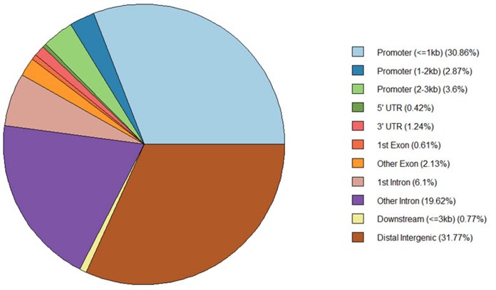
Visualization of genomic annotation (step 7-4)
The ‘annotatePeak’ function assigns peaks to genomic annotation in the “annotation” column of the output, which includes whether a peak is in the TSS, exon, 5′ untranslated region (UTR), or 3′ UTR or intronic or intergenic. The ‘plotAnnoPie’ function provides a pie chart of peak annotations by genomic region (Fig. 5). The distribution of genomic annotation can also be visualized by a histogram (Fig. 6).
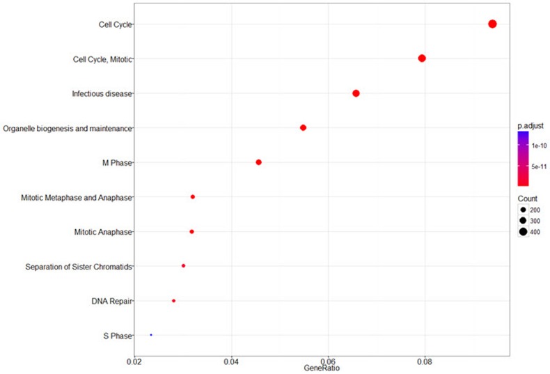
Functional enrichment analysis (step 7-5)
The annotated genes can be used as an input for functional enrichment analysis. The ‘seq2gene’ function changes peak information into gene information, which is used by the ‘enrichPathway’ function for pathway enrichment analysis (Fig. 7).
Discussion
ChIP-Seq is one of major applications using next-generation sequencing technology and provides valuable information on DNA-protein interactions and epigenomic modifications. Due to its high volume of sequence data, most ChIP-Seq data analysis is performed in Unix/Linux or equivalent environments (e.g., Mac OS X). Considering that the Microsoft Windows operating system (OS) still dominates the market share of the PC OS, it would be helpful to have a ChIP-Seq data analysis pipeline that can be run on Windows OS without the use of a Unix-like OS environment.
In this regard, R/Bioconductor provides an excellent opportunity to make an analysis pipeline in an OS-independent manner. First, R/Bioconductor is available for all major platforms (Windows, Mac OS X, and most Linux). Second, most R/Bioconductor packages and scripts can be run across different OS platforms without any modifications. Third, the Bioconductor is an open-source, interdisciplinary, and collaborative software project for the analysis and comprehension of high-throughput data in genomics and molecular biology and provides a lot of useful packages for genomic data analysis [15]. Thus, many useful analysis pipelines can be constructed by deliberately selecting adequate packages among thousands of available high-quality packages. Fourth, R/Bioconductor provides many sophisticated statistical analysis and visualization tools. Indeed, R/Bioconductor is one of the most versatile and advanced visualization systems; so, many high-quality plots in the scientific community are produced using R/Bioconductor.
In this work, we presented a ChIP-Seq data analysis pipeline using only four Bioconductor packages. The entire workflow took only about 2 h in the Windows 7 OS with two Intel i7 quad-cores (3.4 GHz) and 16 GB RAM. Thus, for ChIP-Seq data analysis, we insist that high-end workstations and servers with UNIX-like environments are not mandatory any longer. With careful selection of packages and tools, it is possible to construct an efficient data analysis pipeline on a PC machine. Although more than 60 packages are available for ChIP-Seq data analysis, we deliberately selected four packages to encompass all the necessary steps of ChIP-Seq data analyses, including trimming, mapping and QC, peak calling, peak annotation, and visualization. However, we acknowledge that many other packages with similar functions are also available and can thus be used to construct alternative data analysis pipelines.
In the next version, we will add an option to choose a peak calling algorithm with various statistical analysis options from diverse programs. We hope that our work will help most biologists perform ChIP-Seq data analysis without setting up additional Unix-like environments.