Nowadays, huge volumes of chromatin immunoprecipitation-sequencing (ChIP-Seq) data are generated to increase the knowledge on DNA-protein interactions in the cell, and accordingly, many tools have been developed for ChIP-Seq analysis. Here, we provide an example of a streamlined workflow for ChIP-Seq data analysis composed of only four packages in Bioconductor: dada2, QuasR, mosaics, and ChIPseeker. ‘dada2’ performs trimming of the high-throughput sequencing data. ‘QuasR’ and ‘mosaics’ perform quality control and mapping of the input reads to the reference genome and peak calling, respectively. Finally, ‘ChIPseeker’ performs annotation and visualization of the called peaks. This workflow runs well independently of operating systems (e.g., Windows, Mac, or Linux) and processes the input fastq files into various results in one run. R code is available at github:
Introduction
Various proteins interact with DNA in the nucleus. These interactions include many essential cellular processes, such as DNA replication, recombination, repair, transcription, and histone modifications [
Along with the development of ChIP-Seq data generation methods, various algorithms, methods, and tools have been developed for various steps during ChIP-Seq data analysis. Now, the standard ChIP-Seq data analysis process consists of a quality check (QC), mapping, peak calling, statistical analysis, annotation, and visualization. There are several well-known tools for these steps: ‘Trim Galore’ is one of the best programs to trim fastq reads, and ‘FastQC’ is also one of the major tools for quality control and pre-processing of fastq files. These tools are found at
The Bioconductor project, which was launched in 2001, now contains more than 2,000 packages that facilitate the analysis and interpretation of high-throughput genomic data. As the Bioconductor project is based on the R statistical language, which is available for all of the major operating systems, most packages in Bioconductor can be run across different operating systems. In this regard, packages in the Bioconductor project provide an excellent platform for developing a streamlined analysis pipeline that can be run independently of platform. In this work, we selected four packages (dada2 [
Methods
Public data download
While most researchers are likely to analyze their own data, some users may download public ChIP-Seq data from repositories, such as Short Read Archive (SRA) and the Encyclopedia of DNA Elements (ENCODE) project data portal. In this paper, we used a dataset from Gene Expression Omnibus (GSE29611; the data can be found at
Description of packages and testing environment
We used only four packages from beginning to end. The list of packages is shown in
Results
Overview of the ChIP-Seq analysis workflow
We propose a ChIP-Seq analysis workflow composed of only four Bioconductor packages (
Setting the R environment and installing libraries to analyze (step 0 to step 1)
First, we provide a short R code to install the Bioconductor-based program. Next, it provides the ‘biocLite’ command to install the necessary package to analyze, the ‘setwd’ command to set up the working directory, and the ‘library’ command to load the package.
(Optional) Data download from public repository (step 2)
We downloaded two samples of the GSE29611 dataset from the European Bioinformatics Institute (EBI) database. We used EBI instead of SRA, as EBI provides both fastq and sra files, while SRA provides only sra files. By ftp protocol, it took about 45 min to download two fastq files from the EBI ftp site.
Trimming the sequencing file (step 3)
fastq file filtering is an important step when dealing with high-throughput sequencing data, because low-quality sequences can contain unexpected and misleading errors; especially, Illumina sequencing quality tends to drop off at the ends of reads, and the initial nucleotides can also be problematic due to calibration issues, such as trimming issues. The ‘dada2’ package can filter and trim a fastq file with the ‘fastqFilter’ function. ‘fastqFilter’ takes an input fastq file and filters it, based on several user-definable criteria, and outputs those reads that pass the filter and their associated qualities to a new fastq file. The main parameters of the ‘fastqfilter’ function are ‘fn’ and ‘fout,’ which indicate the path to the input fastq file and to the output file. Additionally, we adjusted the ‘compress’ option to ‘TRUE,’ because we use the compressed fastq file for analysis.
Sequence alignment (step 4)
The first step in ChIP-Seq data analysis is to align fastq files to a reference genome. The names of fastq files and the reference genome information (either a fasta file or BSgenome package) should be provided. As mapping is a time-consuming job, parallel processing using multiple cores is highly recommended. In R, parallel programming is supported by the 'BiocParallel' package, found at
Quality check (step 5)
The next step after sequence alignment is the QC of the aligned reads. The QC is performed by the ‘qQCReport’ function of the qAlign package. It samples a random subset of sequences and alignments from each sample or an input file and generates a series of diagnostic plots for estimating data quality by various methods. The output consists of seven plots. The main plot is shown in
Peak calling (step 6)
For ChIP-Seq peak calling, we chose the ‘mosaics’ package, which uses an adaptive and robust statistical approach; ‘mosaics’ is an acronym of “Model-Based One- and Two-sample Analysis and Inference for ChIP-Seq data.” It implements a flexible parametric mixture modeling approach for detecting peaks—e.g., enriched regions—in one-sample (ChIP sample) or two-sample (ChIP and matched control samples) ChIP-Seq data. It can account for mappability and GC content biases that arise in ChIP-Seq data [
Calling of sharp peaks (steps 6-2 to 6-5)
For peak calling, mosaics first constructs bin-level files from aligned read files for modeling and visualization. The ‘infile’ argument indicates the name of the aligned files, and the ‘fileFormat’ argument indicates the data format of the ‘infile.’ Also, several arguments should be provided: ‘bychr,’ ‘PET,’ ‘fragLen,’ ‘binsize,’ and ‘capping.’ The meaning of each argument is given in ‘constructing separate bin-level file for each chromosome,’ ‘paired-end tag,’ ‘average fragment length,’ ‘size of bins,’ and ‘maximum number of reads allowed to start at each nucleotide position,’ respectively [
Calling of broad peaks (
We provide another version of R code for calling broad peaks (Supplementary Methods,
Annotation and visualization (step 7)
The main input format for the ChIPSeeker package [
ChIP peaks coverage plot (Step 7-2)
The ‘Covplot’ function calculates the coverage of peak regions over chromosomes and generates a figure (
Heatmap and average profiling of chip peaks binding to transcription start site regions (
First, transcription start site (TSS) regions are prepared by invoking the ‘getPromoter’ function. Then, peaks are mapped to the TSS regions, generating tagMatrix. The ‘tagHeatmap’ function plots the heatmap based on the tagMatrix data. The ‘plotAvgProf’ function plots the average profile of the peaks binding to TSS regions (i.e., 5′ to 3′) based on read count frequency.
Peak annotation (step 7-4)
The TSS region, defined by default from −3 kb to +3 kb; the Txdb, and the corresponding annoDb of interest (here, Homo sapiens) should be provided for gene annotation. Then, the annotatePeak function generates annotation information for the given input. Basically, the position and strand information of the nearest genes are reported. The distance from the peak to the TSS of the nearest gene is also reported. The genomic region of the peak is reported in the annotation column. Since some annotations may overlap, the ‘annotePeak’ package adopts the following priority in the genomic annotation: Promoter → 5′ UTR → 3′ UTR → Exon → Intron → Downstream → Intergenic.
Visualization of genomic annotation (step 7-4)
The ‘annotatePeak’ function assigns peaks to genomic annotation in the “annotation” column of the output, which includes whether a peak is in the TSS, exon, 5′ untranslated region (UTR), or 3′ UTR or intronic or intergenic. The ‘plotAnnoPie’ function provides a pie chart of peak annotations by genomic region (
Functional enrichment analysis (step 7-5)
The annotated genes can be used as an input for functional enrichment analysis. The ‘seq2gene’ function changes peak information into gene information, which is used by the ‘enrichPathway’ function for pathway enrichment analysis (
Discussion
ChIP-Seq is one of major applications using next-generation sequencing technology and provides valuable information on DNA-protein interactions and epigenomic modifications. Due to its high volume of sequence data, most ChIP-Seq data analysis is performed in Unix/Linux or equivalent environments (e.g., Mac OS X). Considering that the Microsoft Windows operating system (OS) still dominates the market share of the PC OS, it would be helpful to have a ChIP-Seq data analysis pipeline that can be run on Windows OS without the use of a Unix-like OS environment.
In this regard, R/Bioconductor provides an excellent opportunity to make an analysis pipeline in an OS-independent manner. First, R/Bioconductor is available for all major platforms (Windows, Mac OS X, and most Linux). Second, most R/Bioconductor packages and scripts can be run across different OS platforms without any modifications. Third, the Bioconductor is an open-source, interdisciplinary, and collaborative software project for the analysis and comprehension of high-throughput data in genomics and molecular biology and provides a lot of useful packages for genomic data analysis [
In this work, we presented a ChIP-Seq data analysis pipeline using only four Bioconductor packages. The entire workflow took only about 2 h in the Windows 7 OS with two Intel i7 quad-cores (3.4 GHz) and 16 GB RAM. Thus, for ChIP-Seq data analysis, we insist that high-end workstations and servers with UNIX-like environments are not mandatory any longer. With careful selection of packages and tools, it is possible to construct an efficient data analysis pipeline on a PC machine. Although more than 60 packages are available for ChIP-Seq data analysis, we deliberately selected four packages to encompass all the necessary steps of ChIP-Seq data analyses, including trimming, mapping and QC, peak calling, peak annotation, and visualization. However, we acknowledge that many other packages with similar functions are also available and can thus be used to construct alternative data analysis pipelines.
In the next version, we will add an option to choose a peak calling algorithm with various statistical analysis options from diverse programs. We hope that our work will help most biologists perform ChIP-Seq data analysis without setting up additional Unix-like environments.
Acknowledgments
This work was supported by grants from the genomics (NRF-2012M3A9D1054670 and NRF-2014M3C9A3068554) programs of the National Research Foundation of Korea, which is funded by the Ministry of Science, ICT, and Future Planning, and the KRIBB Research Initiative.
Supplementary materials
Supplementary data including 11 figures and Supplementary methods can be found with this article online at
Supplementary Methods
Calling of broad peaks (step 6 in broad peak script)
Supplementary Fig. 1
Nucleotide frequency. These plots show the frequency of A, C, G, T, and N bases by position in the input reads.
Supplementary Fig. 2
Duplication level. The most frequent sequences are listed; at the same time, these plots show the fraction of reads observed at different duplication levels for each sample.
Supplementary Fig. 3
Mapping statistics. It shows the fraction of reads that were the portion of mappable and unmappable to the reference genome. The percentages of mapped reads were 79.5% and 77.7%, respectively.
Supplementary Fig. 4
Library complexity. It shows the fractions of unique and non-unique read alignment positions. This measure is not independent of the total number of reads in a library. The percentages of unique mapped reads are 85.7% and 93.7%, respectively.
Supplementary Fig. 5
Mismatch frequency. It shows the frequency and position of mismatches in the alignments against the reference genome.
Supplementary Fig. 6
Mismatch type. It shows the frequency of read bases that caused mismatches in the alignments to the reference genome, separately for each genome base.
Supplementary Fig. 7
Coverage plot. Coverage plot visualizes the broad peak locations over the whole genome.
Supplementary Fig. 8
(A) Heatmap of chromatin immunoprecipitation (ChIP) binding to transcription start site (TSS) regions. (B) Average profile of ChIP peaks binding to TSS regions. It shows the read count frequency of the broad peak sample in the range from −3000 bp to +3000 bp.
Supplementary Fig. 9
Pie chart of different genomic regions. UTR, untranslated region.
Supplementary Fig. 10
UpSet plot. UTR, untranslated region.
Supplementary Fig. 11
Functional enrichment analysis. It identifies predominant biological themes among the nearest genes associated with the broad peak by incorporating biological knowledge provided by biological ontologies.
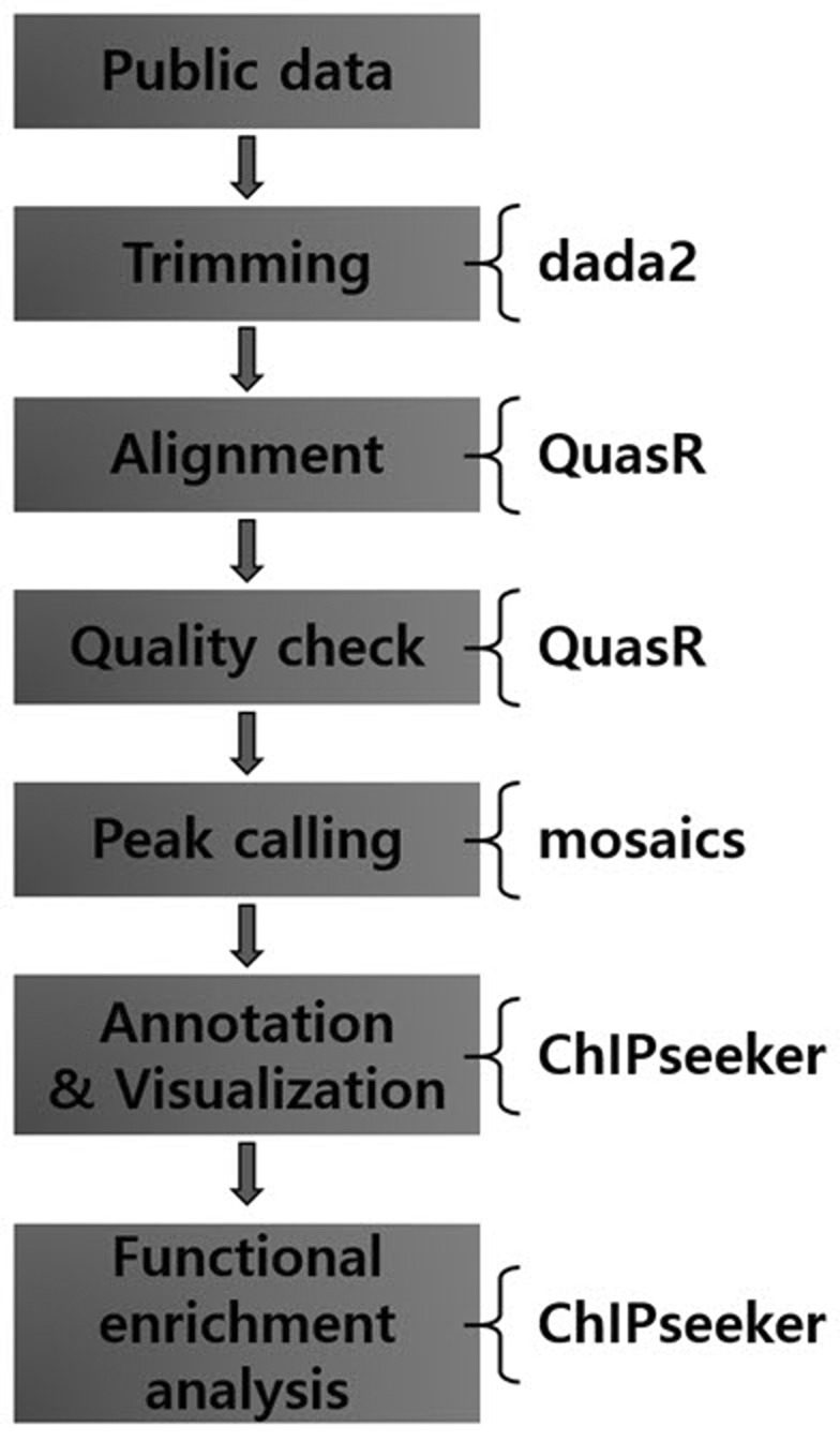
Workflow of chromatin immunoprecipitation-sequencing (ChIP-Seq) data analysis using Bioconductor packages. Four packages are used in this workflow. The ‘dada2’ package performs the trimming of high-throughput sequencing file. The ‘QuasR’ package performs alignment and quality check. The ‘mosaic’ package, which is the core of this workflow, performs the peak calling step. The last package, ‘ChIPseeker,’ performs annotation, visualization, and functional enrichment analysis.
Boxplot of the quality score distribution per base position in reads. It shows the distribution of the base quality values for each position from the input sequence. In this figure, both the control sample and IP sample have very high quality scores.
Coverage plot. It visualizes the peak locations over the whole genome. It is made for calculating the coverage of peak regions over chromosomes.
(A) Heatmap of chromatin immunoprecipitation (ChIP) binding to transcription start site (TSS) regions. It shows the profile of ChIP peaks binding to TSS regions, which are defined as the flanking sequence of TSSs. (B) Average profile of ChIP peaks binding to TSS regions. The average profile of the ChIP peaks is a graph showing the read count frequency in the range from –3000 bp to +3000 bp. Since the H3K4me3 state is a promoter marker, the read count frequency is high in the TSS region.
Pie chart of different genomic regions. There are various parts, including distance promoter and two untranslated regions (UTRs). In particular, the distal intergenic region and the promoter region for 1−2 kb are dominant in the analysis above.
UpSet plot. Matrix layout for all interactions of 7 regions, sorted by size. Dark circles in the matrix indicate sets that are part of the intersection. UTR, untranslated region.
Functional enrichment analysis. It identifies predominant biological themes among the nearest genes by incorporating biological knowledge provided by biological ontologies. It shows results in the gene region from –1000 to +1000 of the transcription start site. The top 3 circles in the figure have p-values of 1.837e-32, 1.970e-29, and 6.854e-21, respectively.
Public datasets used in ChIP-Seq data analysis
| Name | SRR number | GSM number | Peak shape |
|---|---|---|---|
| HeLa control | SRR227391 | GSM733659 | - |
| HeLa H3K4me3 | SRR227441 | GSM733682 | Sharp |
| HeLa H3K27me3 | SRR227473 | GSM733696 | Broad |
ChIP-Seq, chromatin immunoprecipitation-sequencing.
Bioconductor packages used in this study
| Package | Version | Description | Reference |
|---|---|---|---|
| dada2 | 1.2.1 | Manipulating sequencing data | [8] |
| QuasR | 1.140 | Quantify and annotate short reads | [9] |
| mosaics | 2.12.0 | Model based on one- and two-sample analysis and inference for ChIP-seq | [10] |
| ChIPseeker | 1.10.2 | ChIP peak annotation, comparison, and visualization | [11] |