


Introduction
Genome-wide association studies (GWAS) have been extensively performed to identify single nucleotide polymorphisms (SNPs) associated with cross-sectional traits, but GWAS on longitudinal traits have been underexplored [1–5]. Longitudinal traits dynamically change over time, controlled by both genetic and environmental factors. Multiple measurements at various time points under varying environmental conditions are collected as longitudinal traits; thus, conducting a GWAS for longitudinal traits requires considering the covariance among observations at all-time points. Multivariate linear mixed models have been widely adopted for longitudinal GWAS, and efficient multivariate algorithms for longitudinal GWAS have been developed to reduce the computational complexity for SNP-inferred kinship matrix [3,6]. Furthermore, several Bayesian methods such as time-varying-coefficient regression [7], a simple regression-based method [8], and a Gaussian process-based model [9] have been developed for analyzing such longitudinal traits.
Recently, for the analysis of longitudinal genetic data, we developed a Bayesian mixed model with a built-in variable selection feature based on a grid-based covariance estimation approach [10]. The proposed Bayesian method modeled multiple candidate SNPs simultaneously and allowed SNP-SNP and SNP-time/environment interactions, enabling us to detect SNPs with time-varying effects that were of great scientific and medical interest. The proposed grid-based approach modeled the covariance structure nonparametrically; not only was this parsimonious in estimating the covariance matrix, but it also enabled the flexible approximation of any type of covariance structure by employing a reasonable number of grid points. The number of grid points was set in advance, but the deviance information criterion (DIC) [11] and simplified Bayesian predictive information criterion (BPIC) [12] can be utilized to select the optimal number of grid points. Through simulation studies, we showed that the proposed Bayesian method using all-time points outperformed the ordinary Bayesian method with one or all-time points, and statistical power increased as the data had more samples, smaller number of SNPs, a lower proportion of causal SNPs, and larger trait-heritability.
In this paper, we analyze longitudinal obesity-related traits such as body mass index (BMI), hip circumference (HIP), waist circumference (WST), and waist-hip ratio (WHR) from Korea Association Resource (KARE) data to further evaluate the proposed Bayesian method. These traits are well-known markers of obesity across all ages and continuously change over time. We first conduct cross-sectional GWAS analysis at each time point and combine the results of the GWAS analysis of all-time points using a meta-analysis based on a trajectory model [13] and a random-effects model [14]. We then apply our Bayesian mixed model to further discover SNPs associated with the traits and SNP-time/environment interactions. The paper is organized as follows. In Methods section, we describe the KARE data, GWAS analysis, meta-analysis and summarize our grid-based Bayesian mixed model for longitudinal genetic data. In the Results section, we present the analysis results for longitudinal obesity-related traits such as BMI, HIP, WST, and WHR from KARE data and evaluate the proposed Bayesian method. We conclude the paper with a discussion on Bayesian longitudinal analysis and future work.
Methods
Study participants
The Korean Genome and Epidemiology Study (KoGES) was a large prospective cohort study that was initiated to solve public health issues and prepare for personalized and preventive health care in Korea [15]. The purpose of the KoGES was to build a genome epidemiological study platform for various researchers and examine the genetic and environmental etiology of complex traits and common diseases such as type 2 diabetes, hypertension, obesity, and metabolic syndrome in Korea. Data collection was initiated in 2001, and follow-up examinations for the participants have been conducted every 2 years. In particular, the availability of GWAS data and repeatedly measured traits in the KoGES Ansan-Ansung study facilitated the identification of genetic variants associated with various disease traits. The GWAS for the KoGES was known as the KARE cohort, which was launched to perform GWAS to discover the underlying genetic variants associated with diverse complex traits and diseases. The KARE data included 10,038 unrelated individuals aged 40–69 years, assembled through the KoGES Ansan-Ansung study, representing urban and countryside populations, respectively [16]. Our analyses utilized the KARE dataset from the baseline (2001–2002) to the sixth (2013–2014) follow-up.
Genotype data
The 10,038 participants in the KARE were genotyped at ~500,000 SNPs using the Affymetrix Genomewide Human SNP array 5.0. For SNP quality control (QC), we removed SNPs with minor allele frequency (MAF)<0.05, genotype calling rates <95%, and Hardy-Weinberg equilibrium p-values <10−6, resulting in 4,518,929 SNPs. For sample QC, we only preserved participants with consistent sex and calling rates >90%, resulting in 9,331 individuals. The SNP QC and sample QC were performed using PLINK (v1.90) [17]. We then imputed the genotyped SNP data using the Beagle 5.0 software [18] after the SNP and sample QCs. We restricted the analysis to Hapmap3 SNPs with MAF >0.05 and imputation R2 >0.80, which consisted of 3,848,960 SNPs.
GWAS analysis
In the GWAS for cross-sectional obesity-related traits such as BMI, HIP, WST, and WHR, we performed linear mixed model (LMM) association analysis implemented in the BOLT-LMM (v2.3) software [19] using genotyped and imputed genetic variants from the KARE data [20]. The current analysis adjusted for age, age squared, sex, drinking, smoking status, and 10 genotype principal components (PCs). In order to obtain independent SNPs (i.e., a smaller number of clumps of correlated SNPs), we reduced the genome-wide scan using the PLINK clumping function based on empirical estimates of linkage disequilibrium (LD) between genetic variants loci (with four main flags: --clump-p1 5e-8 --clump-p2 1e-5 --clump-r2 0.1 --clump-kb 1000). The clumping procedure found index SNPs (p < 5 × 10⁻⁸) that were independent from each other and formed clumps of other SNPs that were located within 1,000 kb from each index SNP and in LD with the index SNP based on r2 > 0.1. Clumps annotated to the same gene were further combined to the clump with the most significant index SNP.
Meta-analysis using trajectory model
To discover SNPs associated with the overall trend and trajectory of phenotypes, we prepared two different longitudinal outcomes (the average and trajectory), which were obtained from longitudinal BMI, HIP, WST, and WHR measurements (baseline to sixth follow-up). To assess the average outcome, we calculated the average BMI, HIP, WST, and WHR measurements over the six time points and then used the average values as the phenotype for GWAS analysis. To assess the trajectory outcome, we utilized the methodology in Gouveia et al. [13] designed to study cognitive trajectories. The LMM function implemented in the R package lme4 [21] was used to obtain the per-individual trajectory for all obesity-related traits. Specifically, we fitted the following mixed model for subject i at time j:
y i j = ( β 0 + u 0 i ) + ( β 1 + u 1 i ) x 1 i j + ∑ h = 2 q β h x h i j + e i j ( i = 1 , … , n , j = 1 , … , 6 )
Meta-analysis using a random-effects model
We utilized two different meta-analysis methods based on a fixed-effects model (Meta-Fixed) and a random-effects model (Meta-Random) to combine GWAS results for cross-sectional traits across all-time points (baseline to sixth follow-up). The Meta-Fixed method, as exemplified by the inverse-variance weighted method [22] and weighted sum-of-z-scores method [22], assumed that the magnitude of the true effects was common or fixed in every GWAS study and did not model heterogeneity. p-values for all GWAS analyses were converted to z-scores and then combined with different weights for each study according to their sample sizes. Meanwhile, the Meta-Random method proposed by DerSimonian and Laird [23] and Lee et al. [14] assumed that the true effect size of each study was sampled from an underlying distribution and modeled heterogeneity, explicitly. The Meta-Random method had two modifications: (1) accounting for correlation among test statistics based on the Lin and Sullivan method [24], and (2) focusing on heterogeneous effects conditioned on the Meta-Fixed method. The Meta-Random method can obtain higher power to detect heterogeneous effects than the Meta-Fixed method and it allows the testing of heterogeneous effect sizes between individual test statistics.
Grid-based Bayesian mixed model
To further discover SNPs associated with traits of interest and SNPs interacting with time/environmental factors, we considered the following Bayesian mixed model:
where yi = (yi1, …, yini)T is an ni × 1 phenotype vector of individual i; μi = μ1ni is an ni × 1 overall mean vector;
x i = ( x i t , x i g , x i g g , x i gt ) N = ∑ i = 1 n n i p i = ( p i 1 T , … , p i n i T ) T p i j = ( 0 ( r - 1 ) T , t r + 1 - t t r + 1 - t r , t - t r t r + 1 - t r , 0 ( k - r - 1 ) T ) p i j = ( 0 ( r - 1 ) T , 1 , 0 ( k - r ) T )
For Bayesian estimation of the mixed-effects model (1), we applied the modified Cholesky decomposition of Chen and Dunson [25] to the k × k covariance matrix D, resulting in the decomposition, D = ΔΨΨTΔ, where Δ is a nonnegative k × k diagonal matrix and Ψ is a k × k lower triangular with 1’s in the diagonal elements. We re-parameterized model (1) as
where bi = (bi1, … bik)T such that bij ~ N(0,1) and
b i j ⊥ b i j ′ ( j ≠ j ′ )
As priors for Δ and Ψ, we defined two vectors δ = (δl : l = 1, …, k)T and ψ = (ψml : m = 2, …, k; l = 1, …, m − 1)T. The prior distribution for δ is
P ( δ ) = ∏ l = 1 k P ( δ l ) = ∏ l = 1 k N + ( δ l ∣ m l 0 , s l 0 2 ) N + ( δ l ∣ m l 0 , s l 0 2 ) N ( δ l ∣ m l 0 , s l 0 2 ) P ( ψ ) = d N ( ψ 0 , R 0 ) b = ( b 1 T , … , b n T ) T P ( b ) = d N ( 0 , I n k ) P ( β a ∣ γ a , σ β 2 ) = d N ( 0 , γ a σ β 2 ) σ β 2 P ( ψ ) = d N ( η 0 , τ 0 2 ) P ( σ 2 ) = d inv - χ 2 ( ν σ , s σ 2 )
The posterior samples can be used to approximate the posterior distribution of the parameters. The posterior inclusion probability of each SNP was calculated using its inclusion proportion in the Markov chain Monte Carlo samples. The Bayes factor (BF) can be calculated to quantify the evidence for the inclusion of a specific SNP against the exclusion of that SNP. Jeffreys [26] and Yandell et al. [27] suggested the following criteria for judging the significance of each SNP: weak support if the BF falls between 3 and 10; moderate support if the BF falls between 10 and 30; and strong support if the BF is larger than 30 (i.e., log2(BF) > 6.8). A critical issue with the proposed Bayesian model was how to choose an optimal number of grid points, k. We achieved the goal by evaluating the goodness of the predictive distributions of our Bayesian models. Spiegelhalter et al. [11] proposed the DIC and Ando [12] developed the BPIC. We select the optimal number of grid points for our model by minimizing the DIC or simplified BPIC scores. The proposed methods were implemented in an R package named Gridbayes [10], which is available for download at https://github.com/wonilchung/GridBayes.
Results
GWAS analysis
We conducted a GWAS analysis of KARE data on longitudinal obesity-related phenotypes such as BMI, HIP, WST, and WHR. Seven covariates (age, age squared, sex, area, drinking, smoking status and 10 genotype PCs) were included in the analysis. Among 9,331 individuals, we selected 4,621 individuals who had no missing values for either phenotypes or covariates. The number of measurements for each individual was six, and thus the total number of observations was 27,726. Hapmap3 SNPs with MAF > 0.05 and imputation R2 > 0.8 were retained for the GWAS analyses, resulting in 3,848,960 SNPs.
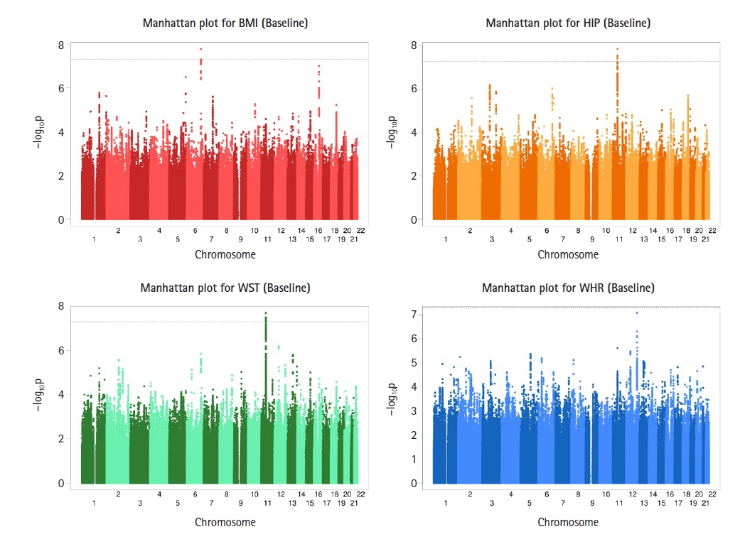
GWAS analyses for cross-sectional obesity-related phenotypes were performed using LMM association analysis implemented in the BOLT-LMM. To assess the cross-sectional outcomes, we analyzed all measurements (baseline to sixth follow-up) separately for each phenotype. Fig. 1 displays Manhattan plots for the baseline BMI, HIP, WST, and WHR measurements and Supplementary Figs. 1–5 in the supplementary materials show the Manhattan plots for the second, third, fourth, fifth, and sixth measurements. Supplementary Figs. 6–11 show the corresponding Quantile-Quantile (Q-Q) plots. For BMI, one SNP on chromosome 6 (baseline) reached GWAS significance (p < 5 × 10⁻⁸), and for HIP, five SNPs on chromosome 11 (baseline), one SNP on chromosome 12 (third follow-up), two SNPs on chromosome 12 (fourth follow-up), and one SNP on chromosome 6 (sixth follow-up) exceeded the threshold for GWAS significance in Supplementary Table 1. For WST, 11 SNPs on chromosome 11 (baseline) and for WHR, 16 SNPs on chromosome 12 (second follow-up), one SNP on chromosome 12 (fifth follow-up), one SNP on chromosome 18 (second follow-up), and one SNP on chromosome 18 (fifth follow-up) reached GWAS significance (see Supplementary Table 1).
Meta-analysis
In order to identify SNPs associated with the overall trend and trajectory of the phenotype, we utilized two types of longitudinal outcomes (average and trajectory), obtained for BMI, HIP, WST, and WHR measurements across consecutive examinations of each individual. For the average outcomes, we calculated the average of all measurements from baseline to sixth follow-up. For the trajectory outcomes, we estimated the per-individual trajectory for all obesity-related traits by fitting a mixed model in the R package lme4 [21]. The model contained a random intercept and a slope for age, as well as other covariates such as age squared, sex, area, and drinking and smoking status. The predicted random slopes of all individuals for age were used as the phenotype for GWAS on trajectory outcomes. We performed BOLT-LMM analyses with these average and trajectory outcomes for four obesity-related traits. Supplementary Fig. 12 shows Manhattan plots for the average outcomes, and Supplementary Fig. 13 shows Manhattan plots for the trajectory outcomes. Supplementary Figs. 14 and 15 show the corresponding Q-Q plots. No GWAS significant SNPs were found for either the average or trajectory outcomes, suggesting that a simple average and simple trajectory of longitudinal outcomes cannot effectively combine the cross-sectional traits; therefore, more sophisticated approaches are necessary.
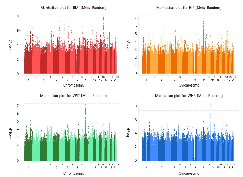
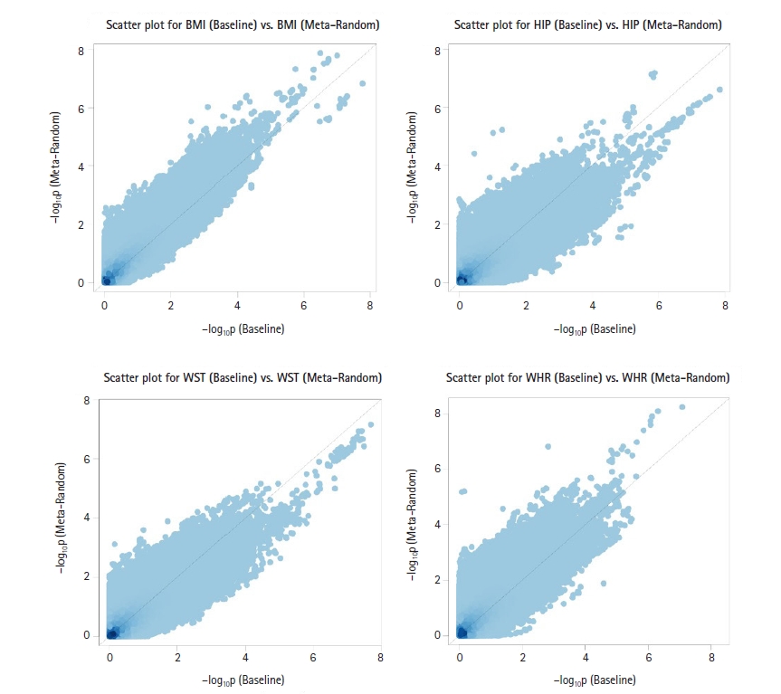
To effectively combine all GWAS results for cross-sectional traits, we performed two different meta-analyses (Meta-Fixed and Meta-Random; see the Methods section) using RE2C software [14]. Because the Meta-Random method accounted for correlation among test statistics for all cross-sectional traits, it would be more appropriate than Meta-Fixed method for our analysis. Supplementary Fig. 16 shows Manhattan plots for the Meta-Fixed method, and Fig. 2 shows Manhattan plots for the Meta-Random method. Supplementary Figs. 17 and 18 show the corresponding Q-Q plots. From the results of Meta-Fixed method, for BMI, two SNPs on chromosome 5 and seven SNPs on chromosome 16 reached GWAS significance, and for WHR, five SNPs on chromosome 12 reached GWAS significance (Supplementary Table 2). From the results of the Meta-Random method, for BMI, two SNPs on chromosome 5 and seven SNPs on chromosome 16 reached GWAS significance, and for WHR, six SNPs on chromosome 12 reached GWAS significance (Supplementary Table 3). Supplementary Fig. 19 shows the scatter plots of −log10(p-value) in GWAS for four longitudinal traits between the Meta-Random method and Meta-Fixed method. As expected, the p-values with the Meta-Random method were smaller than those obtained with the Meta-Fixed method, but there was reasonable concordance between them. In Fig. 3, it can be seen that p-values of the Meta-Random method were more significant than those of the baseline analysis in general.
Bayesian analysis
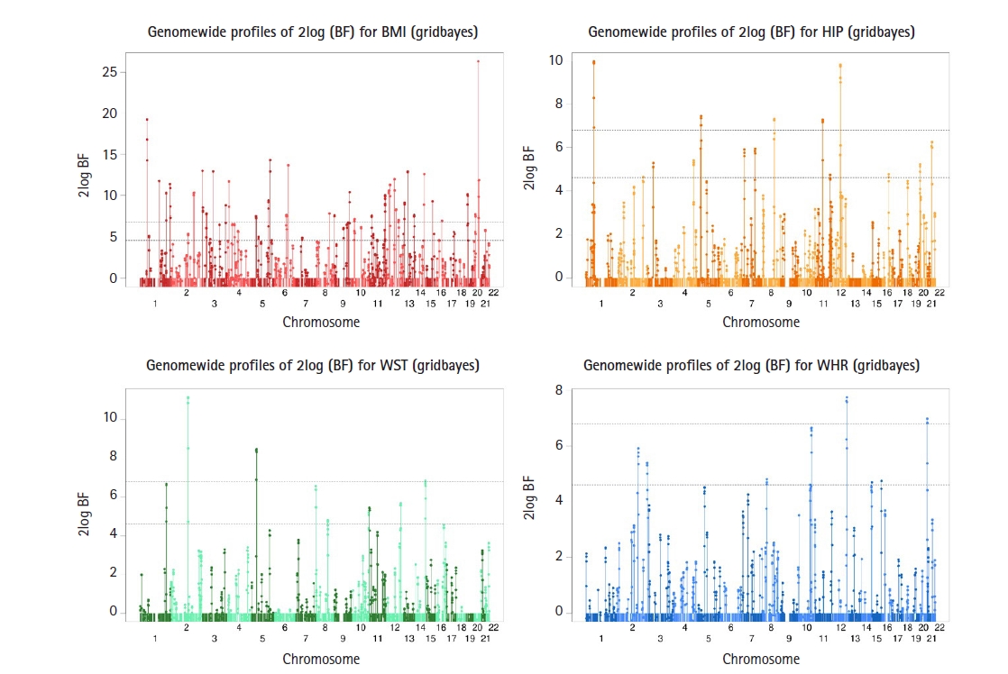
For our Bayesian analysis, a subset of SNPs was selected using LD clumping analysis based on the results of the Meta-Random method to only include SNPs that are not highly correlated with each other (with correlation < 0.5 to avoid multicollinearity). For our Bayesian analysis, we picked a list of the 4,124 SNPs from the LD clumping analyses (option: --clump -kb 250 −p1 0.001 −p2 0.01 −r2 0.5) using PLINK (v1.90) based on summary statistics from the Meta-Random analysis for the four obesity-related traits. Again, our Bayesian analysis included age, age squared, sex, area, drinking, smoking status, and 10 genotype PCs as covariates. The number of grid time points was set to 3 for the analysis based on the DIC and simplified BPIC scores with a different number of grid points (results not shown). Fig. 4 shows the one-dimensional genome-wide profiles of 2log(BF) for the combined effects (main, epistasis, and SNP-age interactions). Based on the criteria suggested in Jeffreys [26] and Yandell et al. [27], we found 112 SNPs with strong signals (i.e., log2(BF) > 6.8) for BMI, 20 SNPs for HIP, 10 SNPs for WST, and 6 SNPs for WHR in Supplementary Table 4. We compared the results of our Bayesian analysis with p-values from the baseline, average, trajectory, and Meta-Random methods and discovered various newly detected novel loci and reasonable concordance among different approaches.
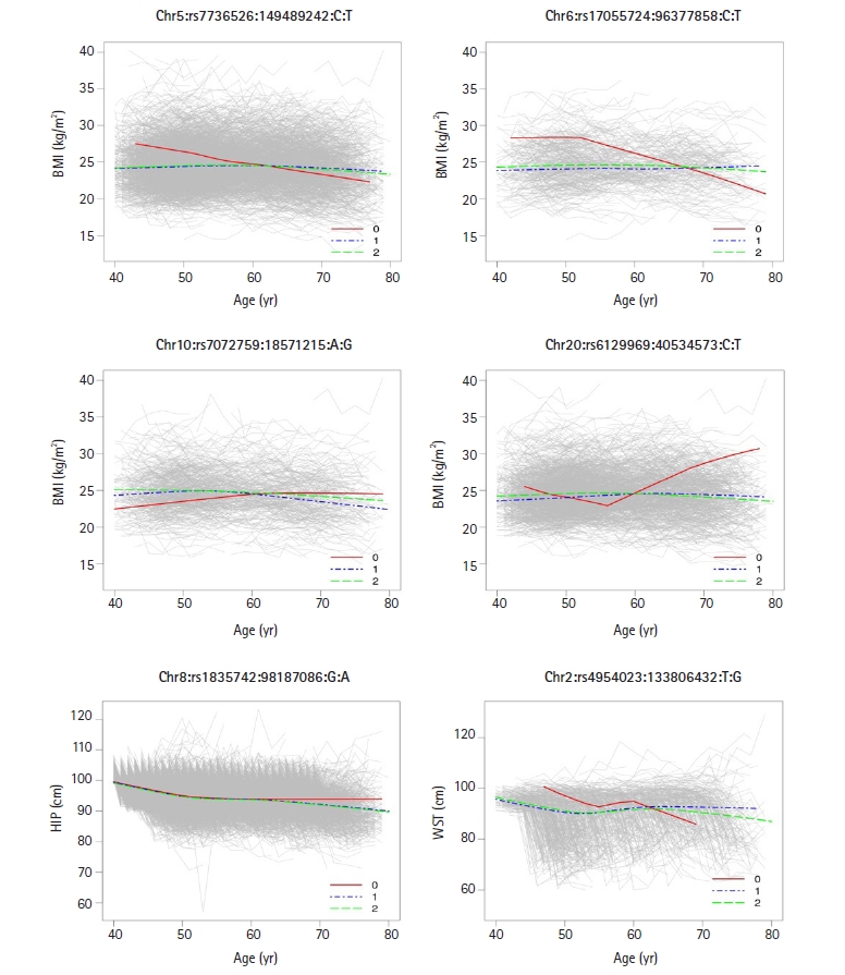
Also, our Bayesian method can discover SNPs interacting with environmental covariates including age, we needed to investigate whether the identified SNPs interacted with age covariate. For SNP-age interaction, we fitted the LMM with each of the four traits (BMI, HIP, WST, and WHR) as a response variable and eight covariates (SNP, age, age squared, sex, area, drinking and smoking status, SNP-age interaction) as predictors:
y i j = ( β 0 + u 0 i ) + ∑ h = 1 7 β h x h i j + e i j ( i = 1 , … , n , j = 1 , … , 6 )
Discussion
In this paper, we performed a meta-analysis based on GWAS results for cross-sectional obesity-related traits such as BMI, HIP, WST, and WHR from KARE data and then applied our Bayesian method to a subset of SNPs selected by meta-analysis to further detect causal SNPs and SNPs with time-varying effects. To obtain the meta-analysis results, we first conducted GWAS analyses on obesity-related traits separately for each time point and then combined all GWAS results based on the average, trajectory, Meta-Fixed, and Meta-Random methods. For our Bayesian analysis, we first selected a subset of SNPs based on Meta-Random results and the LD clumping analyses and then applied our Bayesian method to those selected SNPs. We found our Bayesian method newly detected various novel loci and there was a reasonable concordance between our Bayesian analysis and the average, trajectory, Meta-Fixed, and Meta-Random methods. We also confirmed that almost 25% of the identified SNPs using our Bayesian method had significant p-values for SNP-age interaction, meaning that our Bayesian method can well detect SNPs interacting with age as well as SNPs associated with traits of interest.
With the limited sample size, we restricted our Bayesian analysis to a subset of SNPs based on the BOLT-LMM analysis and LD clumping analysis. With a sufficient sample size, our method can be applied to all available SNPs. We are currently developing a parallel computing algorithm based on a message passing interface to execute multiple groups of SNPs simultaneously. This will make it feasible to apply our method to large-sample GWAS data.
One limitation of the proposed Bayesian model is its interpretability. It cannot readily conclude whether the identified SNPs had main effects and/or interactions with other covariates including time. Novel findings need to be further evaluated to elucidate their mode of action, as we performed the analysis for SNP-age interaction. If the number of identified SNPs is small, we can estimate the effect of each genotypic combination, which we can use to interpret the genetic mode. Our Bayesian model for GWAS data relied on a set of preselected SNPs. How to select a good set of SNPs, especially those with low marginal effects but high interactions with other SNPs or environmental factors, is challenging and deserves further investigation.